Usage example
This is a basic example which shows a workflow to assess wildfire exposure to a community using multiple functions from the fireexposuR package. The package automates the methods within various research products which can be accessed through the following links:
Data preperation
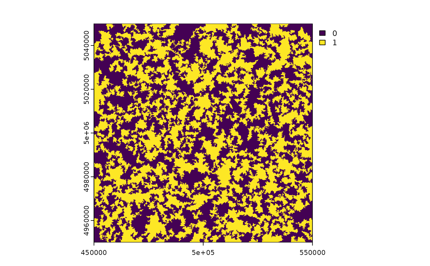
First, some example data will be generated for an imaginary town:
library(terra)
#> terra 1.7.83
# read example hazard data ----------------------------------
filepath <- "extdata/hazard.tif"
haz <- terra::rast(system.file(filepath, package = "fireexposuR"))
# read example AOI
filepath <- "extdata/builtsimpleexamplegeom.csv"
g <- read.csv(system.file(filepath, package = "fireexposuR"))
aoi <- terra::vect(as.matrix(g), "polygons", crs = haz)
# generate random points
pts <- terra::spatSample(aoi, 200)
#' # ----------------------------------------------------------
This example data represents the sort of data that would be pre-prepared by a user for the assessment.
Compute exposure
Now, we will use the hazard data to compute the exposure to long-range ember transmission.
library(fireexposuR)
exp <- fire_exp(haz, tdist = "l")
#> Warning in rgl.init(initValue, onlyNULL): RGL: unable to open X11 display
#> Warning: 'rgl.init' failed, running with 'rgl.useNULL = TRUE'.
Visualize exposure
Once we have an exposure raster the rest of the package functions can
be used to visualize it in different ways. For a landscape, we can map
exposure with a continuous scale with
fire_exp_map_cont():
fire_exp_map_cont(exp)
#> <SpatRaster> resampled to 501264 cells.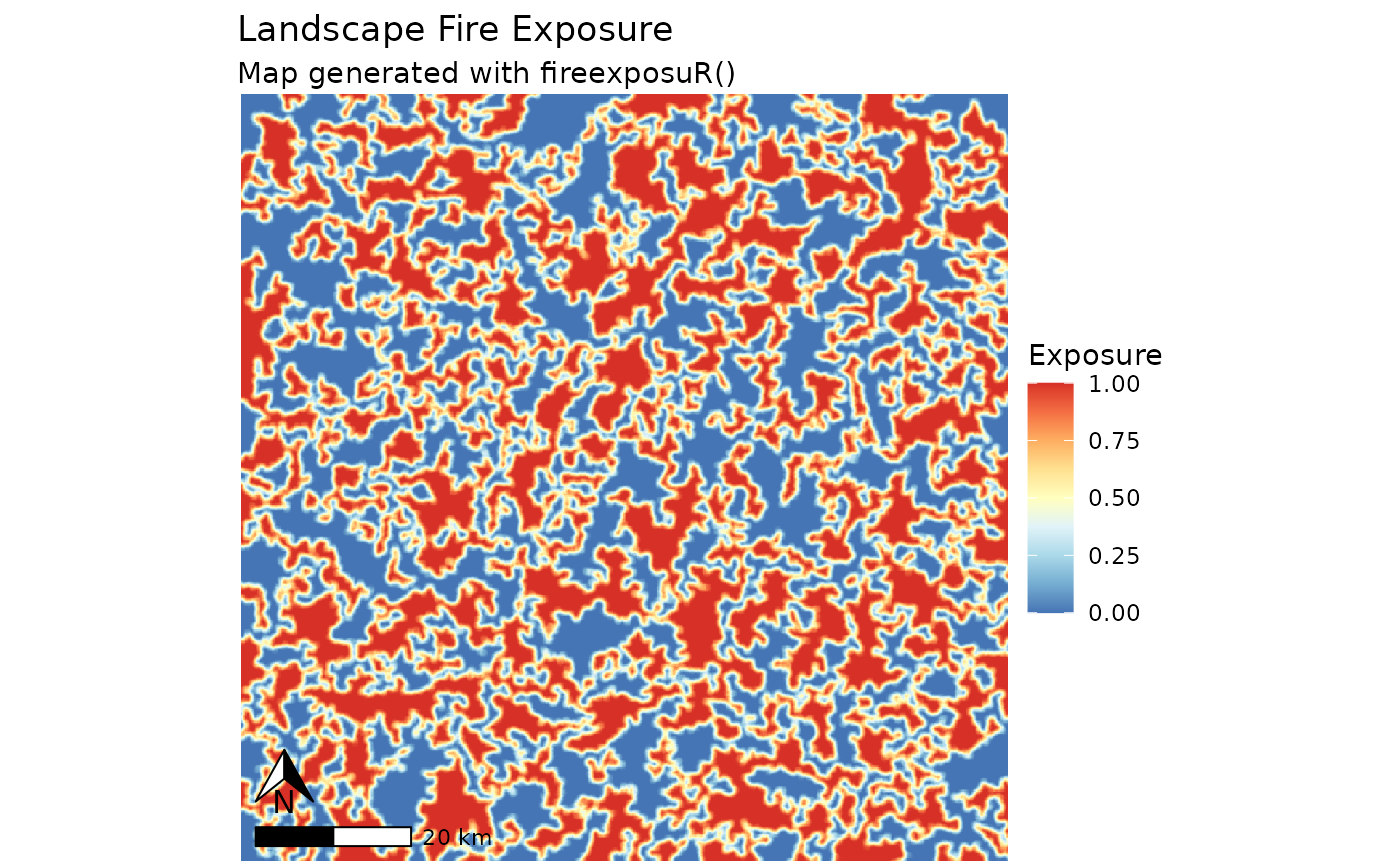
We can also see how that exposure is distributed within the built
environment with exposure classifications in an area of interest with
fire_exp_map_class().
Note: our imaginary town is in the middle of the Pacific Ocean so the base map does not provide further reference.
fire_exp_map_class(exp, classify = "local", aoi)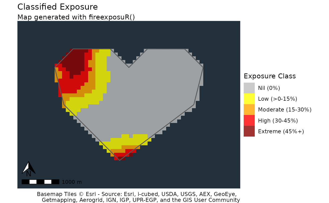
This map gives us a better understanding of areas of the town that
could be fire entry points. We can also summarize the area with
fire_exp_summary() if we want to know the proportional
distributions of each class.
fire_exp_summary(exp, classify = "local", aoi)
#>      class npixels       prop  aream2 areaha
#> 1      Nil     595 0.70749108 5950000    595
#> 2      Low      90 0.10701546  900000     90
#> 3 Moderate      54 0.06420927  540000     54
#> 4     High      58 0.06896552  580000     58
#> 5  Extreme      44 0.05231867  440000     44
We also have data for the values within the built environment, for which we can map or summarize in a table as well.
# extract exposure to the values feature
vals_ext <- fire_exp_extract(exp, pts)
# summary table
fire_exp_extract_vis(vals_ext, classify = "local")
#>   scale method    class   n  prop
#> 1 local  Point      Nil 144 0.720
#> 2 local  Point      Low  21 0.105
#> 3 local  Point Moderate  12 0.060
#> 4 local  Point     High  13 0.065
#> 5 local  Point  Extreme  10 0.050

# map
fire_exp_extract_vis(vals_ext, classify = "local", map = TRUE)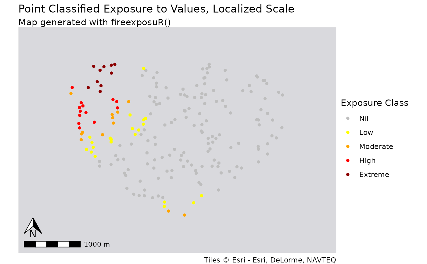
With this information, the community has now identified 12 structures that are extremely exposed to long-range embers from the landscape in the northwest of the community. This could be a potential area to prioritize wildfire mitigation strategies.
Directional vulnerability
Our make believe town may also wish to assess the directional vulnerability to wildfire towards their community. This assessment identifies linear pathways of exposure from the landscape toward a value.
Note: our imaginary town is in the middle of the Pacific Ocean so the base map does not provide further reference.
transects <- fire_exp_dir(exp, aoi)
fire_exp_dir_plot(transects, aoi, map = TRUE)
#> <SpatRaster> resampled to 501120 cells.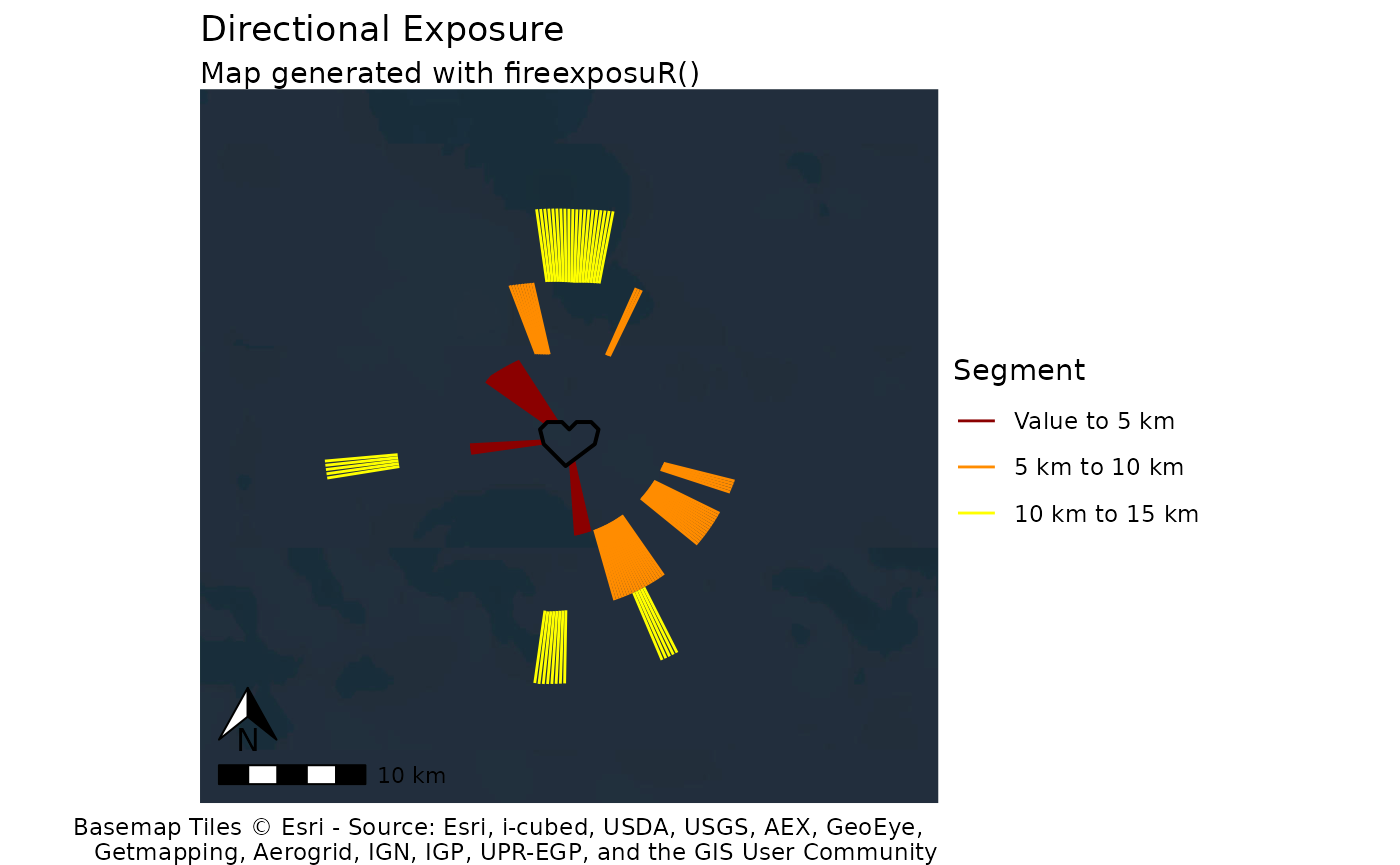
Now we can see that although the northwest corner of the town is a potential entry point, the pathway to that location is only viable from 5 kilometers out. The southeast pathway might be a more concerning pathway because it covers the full 15 kilometers. Depending on local knowledge, this assessment could identify further areas of concern. For example, if the region has consistent patterns of southwest winds it may be a priority area for fuel reduction treatments. Or perhaps there is a popular outdoor recreation area to the northwest close to the community, in which case the shorter pathway might be more of a concern if there is increased human ignition potential in that area.
